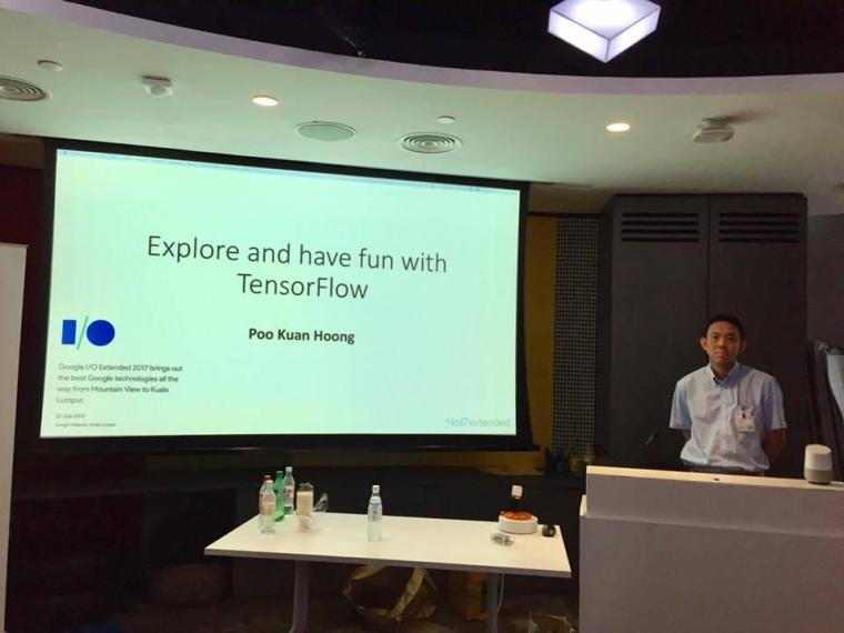
Completed my talk – ‘Explore and Have Fun with TensorFlow: Classifying Cats and Dogs with Transfer Learning” at Google I/O 2017 Extended Kuala Lumpur.
Slides and code are available from my Github.
Data Science, Big Data, R, Machine Learning, Hadoop, Analytics
Completed my talk – ‘Explore and Have Fun with TensorFlow: Classifying Cats and Dogs with Transfer Learning” at Google I/O 2017 Extended Kuala Lumpur.
Slides and code are available from my Github.
Malaysia R User Group Meetup at Microsoft Malaysia, 13th July 2017. Talk entitled “Deep Learning with R”
Slides and demo code are available here: http://github.com/kuanhoong/deeplearning-r
TensorFlow and Deep Learning Malaysia Meetup held at ASEAN Data Analytics Exchange (ADAX), 6th July 2017. Talk entitled ” Explore and Have Fun with TensorFlow: An Introductory to TensorFlow”.
Slides and demo code are available here: http://bit.ly/TensorFlowMY
Three ways to simply paste characters or URLs by using the paste, paste0 and sprintf functions.
x<-"a"
y<-"b"

#paste
paste(x,y)
[1] "a b"

#paste0
paste0(x,y)
[1] "ab"

#paste current working directory to /output/results/
paste0(getwd(),"/output/results")
[1] "C:/Users/Kuan/output/results"

#sprintf
file <-"test.xls"
action <-"read and written"
user<-"Kuan Hoong"
message(sprintf("On %s, the file \"%s\" was %s by %s", Sys.Date(), file, action, user))

On 2016-11-07, the file "test.xls" was read and written by Kuan Hoong
It is easier to use paste0 or paste instead of sprintf as you don’t need to think about the types of arguments being passed.
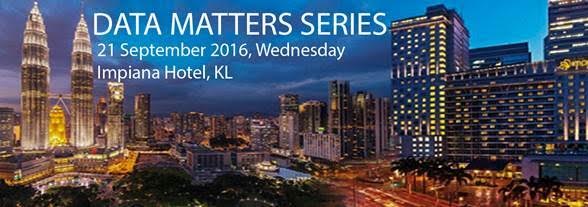
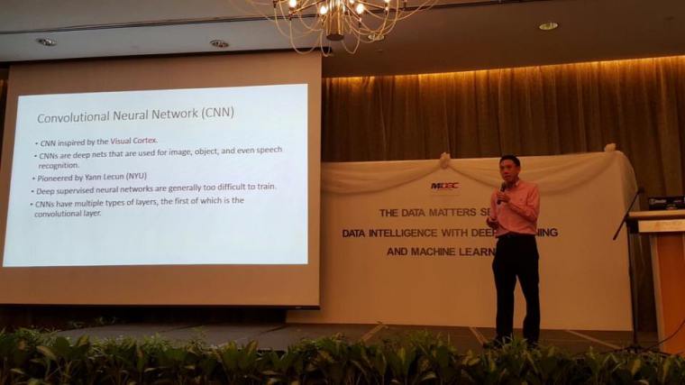
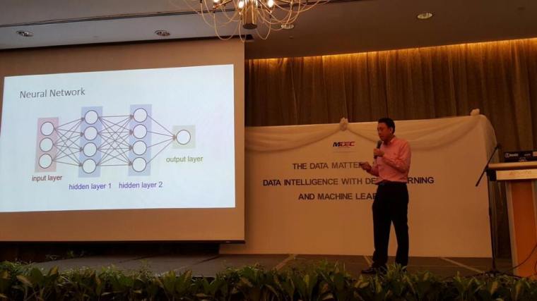
MDEC The Data Matters Series – Data Intelligence with Deep Learning and Machine Learning, 21st September 2016 at Impiana KLCC Hotel, Kuala Lumpur.
Mastering deep learning accordingly positions you at the very forefront of one of the most promising, innovative, and influential emergent technologies, and opens up tremendous new career opportunities. For Data Analysts, Data Scientists, Machine Learning Engineers, and students in a Machine Learning/Artificial Intelligence curriculum, this represents a rarefied opportunity to enhance your Machine Learning portfolio with an advanced, yet broadly applicable, collection of vital techniques.
| Time | Agenda |
| 8.00am – 9.15am | Registration & Breakfast |
| 9.15am – 10.15am | Machine Learning: An Introduction and Overview of Use within Data Science, Dr David Hardoon, Azendian Solutions Pte Ltd |
| 10.15am – 10.45am | Morning Break |
| 10.45am – 11.45pm | Machine Learning & Deep Learning: A Primer by Dr.Poo Kuan Hoong, Multimedia University |
| 11.45am – 12.15pm | Introduction to Deep Learning & Application by Dr Ettikan Kandasamy Karuppiah, NVIDIA |
| 12.15pm – 2.00pm | Lunch |
| 2.00pm – 3.00pm | Deep Learning Use Cases by Terence Chan, NVIDIA |
| 3.00pm – 4.30pm | Deep Learning Hands-On by Mr Nickolas Walker & Dr Ettikan, NVIDIA |
| 4.30pm – 5.00pm | Presentation of token of appreciation and end of event with light refreshment |
Often after the upgrade of R Base, there is a need to install back all the previously installed packages. Here is a simple code to reinstall all the necessary R packages to keep you up and running. The script will check whether the required packages have been installed, if not, it will install them accordingly.
#create a function to check for installed packages and install them if they are not installed
install <- function(packages){
  new.packages <- packages[!(packages %in% installed.packages()[, "Package"])]
  if (length(new.packages))
    install.packages(new.packages, dependencies = TRUE)
  sapply(packages, require, character.only = TRUE)
}

# usage
required.packages <- c("ggplot2", "dplyr", "reshape2", "devtools", "shiny", "shinydashboard", "caret","randomForest","gbm","tm","forecast","knitr","Rcpp","stringr","lubridate","manipulate","Scale","sqldf","RMongo","foreign","googleVis","XML","roxygen2","plotly","parallel","car")
install(required.packages)
Checkout the following posts:
The MNIST database consists of handwritten digits. The training set has 60,000 examples, and the test set has 10,000 examples. The MNIST database is a subset of a larger set available from NIST. The digits have been size-normalized and centered in a fixed-size image. The original NIST’s training dataset was taken from American Census Bureau employees, while the testing dataset was taken from American high school students. For MNIST dataset, half of the training set and half of the test set were taken from NIST’s training dataset, while the other half of the training set and the other half of the test set were taken from NIST’s testing dataset.
For the MNIST dataset, the original black and white (bilevel) images from NIST were size normalized to fit in a 20×20 pixel box while preserving their aspect ratio. The resulting images contain grey levels as a result of the anti-aliasing technique used by the normalization algorithm. the images were centered in a 28×28 image (for a total of 784 pixels in total) by computing the center of mass of the pixels, and translating the image so as to position this point at the center of the 28×28 field.
Deep learning is still fairly new to R. The main purpose of this blog is to conduct experiment to get myself familiar with the ‘h2o’ package. As we are know, there many machine learning R packages such as decision tree, random forest, support vector machine etc. The creator of the h2o package has indicted that h2o is designed to be “The Open Source In-Memory, Prediction Engine for Big Data Science”.
Step 1: Load the training dataset
In this experiment, the Kaggle pre-processed training and testing dataset were used. The training dataset, (train.csv), has 42000 rows and 785 columns. The first column, called “label”, is the digit that was drawn by the user. The rest of the columns contain the pixel-values of the associated image.
Each pixel column in the training set has a name like pixelx, where x is an integer between 0 and 783, inclusive. To locate this pixel on the image, suppose that we have decomposed x as x = i * 28 + j, where i and j are integers between 0 and 27, inclusive. Then pixelx is located on row i and column j of a 28 x 28 matrix, (indexing by zero).
train <- read.csv ( "train.csv")
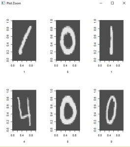
The hand written images are rotated to the left. In order to view some of the images, rotations to the right will be required.
# Create a 28*28 matrix with pixel color values
m = matrix(unlist(train[10,-1]), nrow = 28, byrow = TRUE)

# Plot that matrix
image(m,col=grey.colors(255))

# reverses (rotates the matrix)
rotate <- function(x) t(apply(x, 2, rev))

# Plot some of images
par(mfrow=c(2,3))
lapply(1:6,
       function(x) image(
         rotate(matrix(unlist(train[x,-1]),nrow = 28, byrow = TRUE)),
         col=grey.colors(255),
         xlab=train[x,1]
       )
)

par(mfrow=c(1,1)) # set plot options back to default
Step 2: Separate the dataset to 80% for training and 20% for testing
Using the caret package, separate the train dataset. Store the training and testing datasets into separate .csv files.
library (caret)
inTrain<- createDataPartition(train$label, p=0.8, list=FALSE)
training<-train.data[inTrain,]
testing<-train.data[-inTrain,]

#store the datasets into .csv files
write.csv (training , file = "train-data.csv", row.names = FALSE)
write.csv (testing , file = "test-data.csv", row.names = FALSE)
Step 3: Load the h2o package
library(h2o)

#start a local h2o cluster
local.h2o <- h2o.init(ip = "localhost", port = 54321, startH2O = TRUE, nthreads=-1)
Load the training and testing datasets and convert the label to digit factor
training <- read.csv ("train-data.csv")
testing  <- read.csv ("test-data.csv")

 # convert digit labels to factor for classification
training[,1]<-as.factor(training[,1])

# pass dataframe from inside of the R environment to the H2O instance
trData<-as.h2o(training)
tsData<-as.h2o(testing)
Step 4: Train the model
Next is to train the model. For this experiment, 5 layers of 160 nodes each are used. The rectifier used is Tanh and number of epochs is 20
res.dl <- h2o.deeplearning(x = 2:785, y = 1, trData, activation = "Tanh", hidden=rep(160,5),epochs = 20)
Step 5: Use the model to predict
#use model to predict testing dataset
pred.dl<-h2o.predict(object=res.dl, newdata=tsData[,-1])
pred.dl.df<-as.data.frame(pred.dl)

summary(pred.dl)
test_labels<-testing[,1]

#calculate number of correct prediction
sum(diag(table(test_labels,pred.dl.df[,1])))
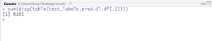
From the model, the accuracy of prediction for the testing dataset is 96.48% (8102 out of 8398).
Step 6: Predict test.csv and submit to Kaggle
Lastly, use the model to predict test.csv and submit the result to Kaggle.
# read test.csv
test<-read.csv("test.csv")

test_h2o<-as.h2o(test)

# convert H2O format into data frame and save as csv
df.test <- as.data.frame(pred.dl.test)
df.test <- data.frame(ImageId = seq(1,length(df.test$predict)), Label = df.test$predict)
write.csv(df.test, file = "submission.csv", row.names=FALSE)

# shut down virtual H2O cluster
h2o.shutdown(prompt = FALSE)

Result from Kaggle shows the accuracy of 96.514%.
Computer scientists have long been inspired by the human brain. The artificial neural network (ANN) is a computational system modeled after the connectivity of human brain. A neural network does not process data in a linear fashion. Instead, information is processed collectively, in parallel throughout a network of nodes (the nodes, in this case, being neurons).
In this simple experiment, it is an attempt to utilize the neural network with R programming.
Step 1: Load the dataset
For this experiment, the Titanic dataset from Kaggle will be used. The sinking of the RMS Titanic is one of the most infamous shipwrecks in history. On April 15, 1912, during her maiden voyage, the Titanic sank after colliding with an iceberg, killing 1502 out of 2224 passengers and crew. In this dataset, the training dataset consists of 891 rows while the testing dataset consists of 418 rows of data. The training dataset consists of labelled survived (YES/NO) rows of data. While the test dataset will be used for prediction and to be submitted to Kaggle for evaluation.
train.data <- read.csv("train.csv")
test.data <- read.csv("test.csv")
Overview of the train.data:
str(train.data)
> str(train.data)
'data.frame':	891 obs. of  12 variables:
 $ PassengerId: int  1 2 3 4 5 6 7 8 9 10 ...
 $ Survived   : int  0 1 1 1 0 0 0 0 1 1 ...
 $ Pclass     : int  3 1 3 1 3 3 1 3 3 2 ...
 $ Name       : chr  "Braund, Mr. Owen Harris" "Cumings, Mrs. John Bradley (Florence Briggs Thayer)" "Heikkinen, Miss. Laina" "Futrelle, Mrs. Jacques Heath (Lily May Peel)" ...
 $ Sex        : chr  "male" "female" "female" "female" ...
 $ Age        : num  22 38 26 35 35 NA 54 2 27 14 ...
 $ SibSp      : int  1 1 0 1 0 0 0 3 0 1 ...
 $ Parch      : int  0 0 0 0 0 0 0 1 2 0 ...
 $ Ticket     : chr  "A/5 21171" "PC 17599" "STON/O2. 3101282" "113803" ...
 $ Fare       : num  7.25 71.28 7.92 53.1 8.05 ...
 $ Cabin      : chr  "" "C85" "" "C123" ...
 $ Embarked   : chr  "S" "C" "S" "S" ...
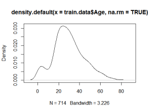
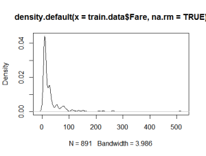
Plot generic density plots to take a look at a few values and to get a better understanding of the data.
plot(density(train.data$Age, na.rm = TRUE))
plot(density(train.data$Fare, na.rm = TRUE))
Step 2: Split the train dataset to training and testing
In order to train the neural network, the train dataset will be divided to 80% for training and 20% for testing. In this case, the library(caret) will be used.
library(caret)
inTrain<- createDataPartition(train.data$Survived,
p=0.8, list=FALSE)
training<-train.data[inTrain,]
testing<-train.data[-inTrain,]
Step 3: Load the nnet package
For this experiment, the nnet package will be used. The nnet package is for feed-forward neural networks with a single hidden layer, and for multinomial log-linear models.
library(nnet)
The nnet package requires that the target variable of the classification (i.e. Survived) to be in two-column matrix — one column for No and the other for Yes — with a 1/0 as appropriate. Convert the Survived column by using the built-in utility class.ind function.
training$Surv = class.ind(training$Survived)
testing$Surv = class.ind(testing$Survived)
Step 4: Train the Model
Fit a neural network for classification purposes:
fitnn = nnet(Surv~Sex+Age+Pclass, training, size=1, softmax=TRUE)
fitnn
summary(fitnn)
Step 5: Evaluate the Model
Evaluate the overall performance of the neural network by looking at a table
of how predictions using the testing data.
table(data.frame(predicted=predict(fitnn, testing)[,2] > 0.5,
actual=testing$Surv[,2]>0.5))
In this evaluation, the probability more than 0.5 will be labelled as “Survived”.
          actual
predicted FALSE TRUE
    FALSE    82   16
    TRUE      9   37
Step 6: Predict the test data
For submission to Kaggle online, use the predict function to predict the survivors for the test data.
*Note: The testing data has been slightly modified by adding column “Survived” to the second column.
predicted=predict(fitnn, test.data) [,2]
predicted[is.na(predicted)]<-0
predicted[predicted >0.5]<-1
predicted[predicted <0.5]<-0
test.data$Survived<-predicted
test.data$Survived
write.csv(test.data[,1:2], "nnet-result1.csv", row.names = FALSE)
Similar to the training, the probability of more than 0.5 will be marked as “Survived (1)” while NA (NA for some passengers’ age) and less than 0.5 will be marked as “Not Survived (0)”
Step 7: Submit to Kaggle
![]()
Submission to Kaggle Online yielded accuracy of 76.077%.
Creating a new R package with pretty simple with RStudio. In a nutshell, packages are the fundamental units of reproducible R code. Generally, packages include reusable R functions, the documentation that describes how to use them, and sample data. As of January 2016, there were over 7,800 packages available on the Comprehensive R Archive Network, or CRAN, the public clearing house for R packages.
Step 1: Create New R Package
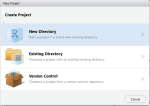
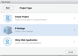
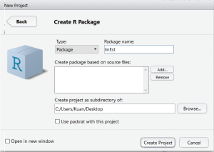
Go to File>New Project>New Directory>R Package. Provide the name for your package and RStudio will create a template for R Package.
The extracted sources of an R package are simply a director on your hard drive. A file named DESCRIPTION with descriptions of the package, author, and license conditions in a structured text format that is readable by computers and by people.
Besides that, there is man/ subdirectory of documentation files, an R/ subdirectory of R code and a data/ subdirectory of datasets.
Step 2: Write the documentation and R Package
Create a new R file for your package which consists of all your R function codes. You may include all your documentation inside the R code. This will be displayed in the R documentation.
Sample of code (modified from this tutorial)
#  linEst.R
#' A simple function which computes the OLS estimate
#' @param x a numeric design matrix for the model
#' @param y a numeric vector of responses
#' @param formula a symbolic description of the model to be fit
#' @return An object of class with list of elements
#' @author Kuan Hoong
#' @details function which computes the OLS estimate
#' @seealso \code{lm}
#' @export

linEst <- function(x, y)
{
  ## compute QR-decomposition of x
  qx <- qr(x)

  ## compute (x'x)^(-1) x'y
  coef <- solve.qr(qx, y)

  ## degrees of freedom and standard deviation of residuals
  df <- nrow(x)-ncol(x)
  sigma2 <- sum((y - x%*%coef)^2)/df

  ## compute sigma^2 * (x'x)^-1
  vcov <- sigma2 * chol2inv(qx$qr)
  colnames(vcov) <- rownames(vcov) <- colnames(x)
  list(coefficients = coef,
       vcov = vcov,
       sigma = sqrt(sigma2),
       df = df)
}
Sample of DESCRIPTION file:
Package: linEst
Type: Package
Title: Minimal R function for linear regression
Version: 1.0
Date: 2016-01-20
Author: Kuan Hoong
Maintainer: Kuan Hoong
Description: This is a demo package

License: GPL-3
LazyData: TRUE
You need to edit the DESCRIPTION file to include all the related information related to your package.
Step 3: Configure Build Tools
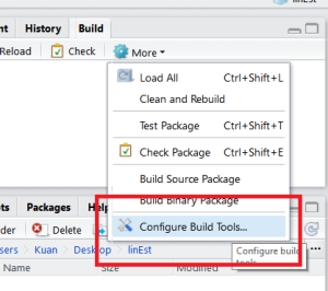
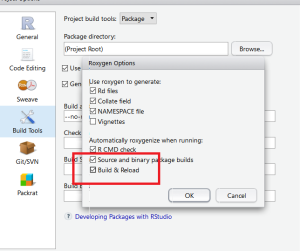
Next step is to configure the Build Tools. Select “Generate Documentation with Roxygen” and in the configuration select “Build & Reload”.
Last time is to click the “Build & Reload” button to build your R Package.
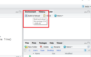
Step 4: Build & Reload
Once your R Package has been successfully built, you may call your package by calling the library.
library(linEst)

#check the description
library(help=linEst)

#read the R Documentation
?linEst
Step 5: Run the library
For example you may run the library with the CATS dataset available from the MASS package.
#to run the package with cats data
data(cats, package="MASS")
linEst(cbind(1, cats$Bwt), cats$Hwt)
Step 6: Submitting to CRAN
Lastly, if you would like to “submit” a package to CRAN, check that your submission meets the CRAN Repository Policy and then use the web form.
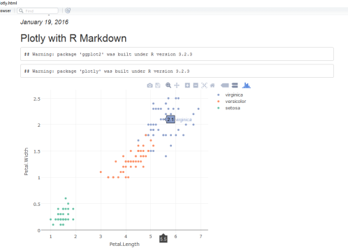
Plotly for R is an interactive, browser-based charting library built on the open source JavaScript graphing library, plotly.js. It works entirely locally, through the HTML widgets framework. Plotly graphs are interactive. You can Click-drag to zoom, shift-click to pan, double-click to autoscale all the graphs.
By default, plotly for R runs locally in your web browser or R Studio’s viewer. You can publish your graphs to the web by creating a plotly account.
To embed plotly plots in R Markdown, simply embed the plotly code into markdown file.
Example:
## Plotly with R Markdown

```{r, plotly=TRUE, echo=FALSE, message=FALSE}
library(ggplot2)
library(plotly)
p <- plot_ly(iris, x = Petal.Length, y = Petal.Width, color = Species, mode = "markers")
p
```
Sample Output: